News Article Recommendation With Contextual Bandit

Recently I read an interesting paper: A Contextual-Bandit Approach to Personalized News Article Recommendation. I noticed its dataset is available, so I thought to play with it. Here, I share a background theory and basic intermediate experimetnal results.

Suppose you are running a local news company that earns most of its advertisement impressions from your website. You want a system that makes a personalized recommendation for an article (item) to each site visitor (user). How do we design such a system? Well, Contextual Bandit (CB) algorithms could be a good option.

Exploration-Exploitation Dillemma

To motivate CB, let us add details to the story. Your workforce is quite big, so you have a constant influx of new items. Your site is also popular, so new users come and go often. Now, learning a recommender system in this setting is tricky. First, we would know very little about the new users and quite nothing about how they relate to existing users (similarity). The same for new items.

One way to resolve it is to passively wait and collect information about new users until we feel confident about their preferences. Then again, the call for a decision is upon us and we cannot serve them a blank page. Another way would be to make bold moves by carefully recommending articles to a new user such that each article effectively decreases the uncertainty about the user preference, all the while thinking about the best recommmendation for the user. Overall, this is called an exploration-exploitation dillemma. The user/item-changing nature makes it hard to apply popular recommendation algorithms like collaborative filtering or content-based filtering. Especially so, when there are not many data points (the cold-start problem). In contrast, Contextual Bandit by design balances between exploration and exploitation.

Multi-armed Bandit

A multi-armed Bandit Problem. Credit: Microsoft Research.

Suppose you are given $k$ actions $\mathcal{A}_k$. At each timestep $t=1,2,\dots$, you take one action $a_t \in \mathcal{A}_k$ and receive a non-negative scalar reward $r_t \sim P_\theta(\cdot \vert a_t)$ where $\theta$ is the unknown parameters of a stationary distribution over rewards. Define the value of taking an action $a_j$ to be $\mu_j = \mathbb{E}_{P_\theta} [R_t \vert A_t = a_j ]$. Define the value of the optimal action $\mu^\star = \arg\max_{j \in [k]} \mu_j$. Define the regret of taking $\delta_j = \mu^\star - \mu_j$. From this, the expected regret after $T$ steps can be defined: $\delta^T = \mathbb{E} [T \mu^\star - \sum_{j \in [k]} n_j \mu_j ]$ where $n_j$ is the number of times $a_j$ was chosen over $T$ steps. Define the action value estimator $Q: \mathcal{A}_k \mapsto [0, \infty]$. We hope to achieve $\mu_j \approx Q(a_j)$. In order to compute an optimal action, we would need to $\arg\max_j Q(a_j)$ (exploitation).

Then, again how do we explore? The general principle of CB for exploration is optimism under uncertainty. That is, if we are not sure about our $Q$ estimate for an action, we intentionally overestimate its action value such that we end up trying it out.

$\epsilon_n$-greedy

We just average all the rewards collected from taking $a_j$ over $T$ steps. $Q_s(a_j) = \bar{r}_j(T) = \frac{1}{n_j}\sum_{t=1}^T \mathbb{I}(a_t = a_j) r_t$. This is a sample mean estimator ($n_j$ estimates from one sample) and as such, it is unbiased. Since the main goal is to discover an optimal action (with the maximum expected reward), we need to try all actions at least once. To explore, we take an action chosen uniformly at random with a small probability $\epsilon$ and otherwise take a greedy decision $\arg\max_j Q(a_j)$. As we explore, we will have reduced enough uncertainty to conclude the optimal action. At that point, exploration would not be needed. Hence, we decay $\epsilon_1, \epsilon_2, \dots$ by a small factor (hyperparameter).

Upper Confidence Bound (UCB)

Suppose for each timestep $t$, we want to construct a confidence interval $c_j(t)= c(t, n_j(t))$ that keeps $\vert Q(a_j) - \mu_j \vert < c_{t,j}$ with a high probability that we can control. Suppose we decide how many steps we will play the game and let it be $n$. Furthermore, we assume in our formulation rewards $R_1, R_2, \dots, R_n$ are i.i.d. We assume the rewards are bounded. Then, using Hoeffding’s inequality, we can upper-bound the probability that our estimate $Q(a_j)$ deviates from the estimand $\mu_j$ by more than any constant $a > 0$ and show the bound can be made arbitrarily small with a large $n$. This leads to $c_j(t) = \sqrt{\frac{\log n}{ n_j(t) }}$ and we solve: $\arg\max_j Q(a_j) + c_j(t)$. Of course, it is awkward to assume we know $n$ a priori. Auer et al¹ proved a more natural bound $c_j(t) = \sqrt{\frac{2 \log t}{n_j(t)}}$.

Thompson Sampling

Thompson Sampling is a Bayesian kid for Multi-Armed Bandit. It follows the typical routine of posterior inference: a) set up a hypothesis (likelihood model) that is assumed to generate observations, b) define a prior over the model parameters, c) using Bayes rule, compute the posterior or the posterior predictive. In our case, we would model $P_\theta (r_t \vert a_t) \approx P_w(r_t \vert a_t)$ and define a prior over $\theta$. For certain combinations of likelihood model and prior that we can write the posterior down in a closed form (conjugate models), the exact inference is tractable. That said, in general, we know an exact Bayesian inference is often intractable because of the evidence in the denominator. I refer the reader to a nice tutorial on Thompson Sampling².

Contextual Bandit

Up until now, our formulation was context-free; it only conditioned on the action (index). Now, suppose for each timestep, we observe an additional random variable about either user or item (=action). Let us define the context at the timestep $t$, $x_{t,a} = \text{concat}(a_t, u_t)$ that depends both on the user context $u_t$ and action $a_t$. The aim is almost the same as before. We are to learn an estimator $Q_w(x_{t,a}) \approx \mathbb{E}[r_t \vert X_{t,a}=x_{t,a}]$.

LinUCB Policy

The algorithm implements a ridge linear regression with UCB. Define the linear estimator $Q_w(x_{t,a}) = w^\top x_t$. Let $D_a \in \mathbb{R}^{n_j \times d}$ denote the design matrix (the training data) and $d$ the dimension of $x_{t,a}$. Let $\mathbf{r}_j \in \mathbb{R}^{n_j}$ the observed rewards corresponding to $D_a$. Assuming we solve a least-squares problem with a ridge regularization ($\lambda=1$), we have a closed-form solution $w^\star = (D_a^\top D_a + I_d)^{-1} D_a^\top r_j$. When elements $r_j$ are conditionally independent given correponding rows in $D_a$, it holds that

$P \left (\, \vert Q_w(x_{t,a}) - \mathbb{E}[ r_t \vert x_{t,a}] \vert \le \alpha \sqrt{ x_t^\top A_a^{-1} x_{t,a}} \,\right ) > 1- \delta$.

where $A_a = (D_a^\top D_a + I_d)^{-1}$ and $\alpha = 1 + \sqrt{\log(2/\delta)/2}$. Thanks to $I_d$, $A_a$ is likely invertible. Inverting a matrix is quite $O(d^3)$ so in practice, we want to solve the linear system periodically as opposed to every step. Finally, we choose $\arg\max_j \big \{ Q_w(x_{t,a_j}) + \alpha \sqrt{ x_{t,a_j}^\top A_{a_j}^{-1} x_{t,a_j}} \big \}$.

The original paper suggests two versions: a disjoint model that learns separate $w_a$ for each action and a hybrid model that has shared parameters across actions. I did not quite like the disjoint model; especially because one must maintain the set of valid actions that can change over time (e.g. new articles coming in and old articles perish). For the experiment (yahoo news), as a simple baseline, I wrote a model that shares all the parameters for all actions. Such a simple linear model may underperform in the high data regime but I expected an okay-level performance in the low data regime.

1
2
3
4
5
6
7
8
9
10
11
12
13
14
15
16
17
18
19
20
21
22
23
24
25
26
27
28
29
30
31
32
33
34
35
36
37
38
39
40
41
42
43
44
45
46
47
48
49
50
51
52
53
54
55
56
57
58
59
60
61
62
63
64
65

class SharedLinUCBPolicy(object):
    """
    unlike the disjoint LinUCB in [1],
    all actions share all parameters.

    [1]: https://arxiv.org/pdf/1003.0146.pdf
    """
    def __init__(self, context_dim, delta=0.2,
                 train_starts_at=500, train_freq=50,
                 batch_mode=False, batch_size=1024
                 ):

        # bias
        self._d = context_dim + 1

        # initialize with I_d, 0_d
        self._A = np.identity(self._d)
        # we will update this every train_freq
        self._A_inv = np.linalg.inv(self._A)

        self._b = np.zeros(self._d)
        self._theta = np.linalg.inv(self._A).dot(self._b)

        self._alpha = 1 + np.sqrt(np.log(2/delta)/2)

        self._t = 0
        self._train_freq = train_freq
        self._train_starts_at = train_starts_at


    def choose_action(self, x_t):
        u_t, S_t = x_t
        # number of actions can change
        n_actions = S_t.shape[0]

        # estimate an action value
        Q = np.zeros(n_actions)
        ubc_t = np.zeros(n_actions)

        for j in range(n_actions):
            # user_context + action_context + bias
            x_t = np.concatenate( (u_t, S_t[j, :], [1]) )

            # compute upper bound
            k_ta = x_t.T.dot(self._A_inv).dot(x_t)
            ubc_t[j] = self._alpha * np.sqrt(k_ta)
            Q[j] = self._theta.dot(x_t) + ubc_t[j]

        a_t = np.argmax(Q)
        self._t += 1

        return a_t

    def update(self, a_t, x_t, r_t):
        u_t, S_t = x_t
        x_t = np.concatenate( (u_t, S_t[a_t, :], [1]) )
        self._A += x_t.dot(x_t.T)
        self._b += r_t * x_t

        if self._t < self._train_starts_at:
            return

        if self._t % self._train_freq == 0:
            self._A_inv = np.linalg.inv(self._A)
            self._theta = self._A_inv.dot(self._b)

Linear Gaussian Thompson Sampling Policy (lgtsp)

This is a Thompson Sampling policy that implements Bayesian linear regression with a conjugate prior. We assume the underlying model (likelihood) satisfies $y_{t,a} = w^\top x_{t,a} + \epsilon$ where $\epsilon \sim N(0, \sigma^2 I_d)$. We define a prior jointly on $w, \sigma^2$ such that $p(w, \sigma^2 ) = p(w | \sigma^2) p(\sigma^2)$ where $p(w_a | \sigma^2)=N(\mu_0, \sigma^2 \Lambda_0^{-1}), \, p(\sigma^2) = \text{inv-gamma}(a_0, b_0)$. The posterior update is well written in wiki. By assumging the initial hyperparam $\mu_0=0$, we can zero out some terms which I did for the experiments. Although the exact posterior update is tractable in this formulation, evaluating a covariance matrix can be too expensive. I noticed it is indeed the bottleneck in my implementation and multivariate_normal ran into a degenerate covariance matrix and failed SVD on it. A better approach would be find a diagonal covariance matrix approximation, which I have not tried out yet. For computational reasons, I collect every data point but update the posterior periodically. I built, again, a shared parameter model across all actions.

1
2
3
4
5
6
7
8
9
10
11
12
13
14
15
16
17
18
19
20
21
22
23
24
25
26
27
28
29
30
31
32
33
34
35
36
37
38
39
40
41
42
43
44
45
46
47
48
49
50
51
52
53
54
55
56
57
58
59
60
61
62
63
64
65
66
67
68
69
70
71
72
73
74
75
76
77
78
79
80
81
82
83
84
85
86
87
88
89
90
91
92
93
94
95
96
97
98
99
100
101
102
103
104
105
106
107
108
109
110
111
112
113
114
115
116
117
118
119
120
121
122
123
124
125
126
127
128
129
130
131
132
133
134
135
136
137
138
139
140
141
142
143
144
145
146
147
148
149
150
151
152
153
154
155
156
157
158
159
160
161
162
163
164
165
166
167
168
169

class SharedLinearGaussianThompsonSamplingPolicy(object):
    """
    A variant of Thompson Sampling that is based on

    Bayesian Linear Regression

    with Inverse Gamma and Gaussian prior
    """

    def __init__(self, context_dim, eta_prior=6.0, lambda_prior=0.25,
                 train_starts_at=500, posterior_update_freq=50,
                 batch_mode=True, batch_size=256, lr=0.01
    ):

        self._t = 1
        self._update_freq = posterior_update_freq
        self._train_starts_at = train_starts_at

        # bias
        self._d = context_dim + 1

        # inverse gamma prior
        self._a_0 = eta_prior
        self._b_0 = eta_prior
        self._a = eta_prior
        self._b = eta_prior

        # conditional Gaussian prior
        self._sigma_sq_0 = invgamma.rvs(eta_prior, eta_prior)
        self._lambda_prior = lambda_prior

        # precision_0 shared for all actions
        self._precision_0 = self._sigma_sq_0 / self._lambda_prior

        # initialized at mu_0
        self._mu = np.zeros(self._d)

        # initialized at cov_0
        self._cov = 1.0 / self._lambda_prior * np.eye(self._d)

        # remember training data
        self._X_t = None

        # for computational efficiency
        # train on a random subset
        self._batch_mode = batch_mode
        self._batch_size = batch_size
        self._lr = lr


    def _update_posterior(self, X_t, r_t_list):
        """
        p(w, sigma^2) = p(mu|cov)p(a, b)
        where p(sigma^2) ~ Inverse Gamma(a_0, b_0)
              p(w|sigma) ~ N(mu_0, sigma^2 * lambda_0^-1)
        """
        cov_t = np.linalg.inv(np.dot(X_t.T, X_t) + self._precision_0)
        mu_t = np.dot(cov_t, np.dot(X_t.T, r_t_list))
        a_t = self._a_0 + self._t/2

        # mu_0 simplifies some terms
        r = np.dot(r_t_list, r_t_list)
        precision_t = np.linalg.inv(cov_t)
        b_t = self._b_0 + 0.5*(r - np.dot(mu_t.T, np.dot(precision_t, mu_t)))

        if self._batch_mode:
            # learn bit by bit
            self._cov = cov_t * self._lr + self._cov * (1 - self._lr)
            self._mu = mu_t * self._lr + self._cov * (1 - self._lr)
            self._a = a_t * self._lr + self._cov * (1 - self._lr)
            self._b = b_t * self._lr + self._cov * (1 - self._lr)

        else:
            self._cov = cov_t
            self._mu = mu_t
            self._a = a_t
            self._b = b_t


    def _sample_posterior_predictive(self, x_t, n_samples=1):
        """
        p(R_new | X, R_old)
        = int p(R_new | params )p(params| X, R_old) d theta

        """

        # 1. p(sigma^2)
        sigma_sq_t = invgamma.rvs(self._a, scale=self._b)

        try:
            # p(w|sigma^2) = N(mu, sigam^2 * cov)
            w_t = np.random.multivariate_normal(
                    self._mu, sigma_sq_t * self._cov
            )
        except np.linalg.LinAlgError as e:
            logger.debug("Error in {}".format(type(self).__name__))
            logger.debug('Errors: {}.'.format(e.args[0]))
            w_t = np.random.multivariate_normal(
                    np.zeros(self._d), np.eye(self._d)
            )

        # modify context
        u_t, S_t = x_t
        n_actions = S_t.shape[0]

        x_ta = [
                np.concatenate( (u_t, S_t[j, :], [1]) )
                for j in range(n_actions)
        ]

        # 2. p(r_new | params)
        mean_t_predictive = [
                np.dot(w_t, x_ta[j])
                for j in range(n_actions)
        ]

        cov_t_predictive = sigma_sq_t * np.eye(n_actions)
        r_t_estimates = np.random.multivariate_normal(
                            mean_t_predictive,
                            cov=cov_t_predictive, size=1
                        )
        r_t_estimates = r_t_estimates.squeeze()

        return r_t_estimates


    def choose_action(self, x_t):
        # p(R_new | params_t)
        r_t_estimates = self._sample_posterior_predictive(x_t)
        act = np.argmax(r_t_estimates)
        self._t += 1

        return act


    def update(self, a_t, x_t, r_t):
        u_t, S_t = x_t
        x_t = np.concatenate( (u_t, S_t[a_t, :], [1]) )

        # add a new data point
        if self._X_t is None:
            X_t = x_t[None, :]
            r_t_list = np.array([r_t])
        else:
            X_t, r_t_list = self._train_data[a_t]
            n = X_t.shape[0]
            X_t = np.vstack( (X_t, x_t))
            r_t_list = np.append(r_t_list, r_t)

        # train on a random batch
        n_samples = X_t.shape[0]
        if self._batch_mode and self._batch_size < n_samples:
            indices = np.arange(self._batch_size)
            batch_indices = np.random.choice(indices,
                                             size=self._batch_size,
                                             replace=False)
            X_t = X_t[batch_indices, :]
            r_t_list = r_t_list[batch_indices]

        self._train_data = (X_t, r_t_list)

        # exploration phase to mitigate cold-start
        if self._t < self._train_starts_at:
            return

        # update posterior prioridically
        n_samples = X_t.shape[0]
        if n_samples % self._update_freq == 0:
            self._update_posterior(X_t, r_t_list)

Neural $\epsilon_n$-Greedy Policy (nueralp)

We fit a simple fully-connected neural network wth stochastic-gradient-based optimizers like RMSProp to the data coming online. It is the same as $\epsilon_n$-Greedy Policy except we use a neural network to represent $Q(x_{t,a})$. Neural networks may be one good way to overcome the limited representation power of the linear models introduced so far. Instead of leaving the exploration to the hyperparameter $\epsilon$, one may keep the Bayesian linear regression formulation and fit a nueral network $g$ such that $y = w^\top z_x + \epsilon, z_x = g(x)$.

Other baselines

• random policy (rp): uniformly at random
• $\epsilon_n$-greedy (egp): sample mean policy + annealing exploration.
• sample mean policy (smp): no exploration.
• optimal policy (opt_p): assumes an oracle that knows the optimal action.

Experiments

Well, that was a review of basic Contextual Bandit algorithms. Now we move on the experiemnts.

Partially-observable Reward Dataset

Here’s a qustion. How do we train the algorithms on a dataset someone else collected for us? So far, our formulation assumed we are learning a policy in an on-policy setting. It means the policy we collect data from (behavior poilcy) is the same as the policy we optimizer (the target policy). In most practical situations, one would have a dataset sampled by a policy and train another policy using the dataset. This realistic setting makes it hard for us to evaluate the true performance of our policy. If a behavior policy always chooses one action among others, we would not have any samples for counterfactuals (=what happens if we had taken other action). This problem is called Off-policy Policy Evaluation and an important research topic.

In an on-policy setting, we can observe the rewards for all actions at will. All it takes is to try the actions we want. In an off-policy setting, however, we cannot directly observe rewards unless the behavior policy that collects data deliver them to us. Then, how do we use such partially observable reward data for training? One naive way to reject any samples where our policy’s action does not match the ation empirically taken by the behavior policy. If we assume a uniform random behavior policy, indeed the performance evaluation would be unbiased. Or we could use an Importance Sampling to obtain an unbiased estimate for the performance. These methods are okay if there are a lot of samples. For the experiment we use the naive rejection method.

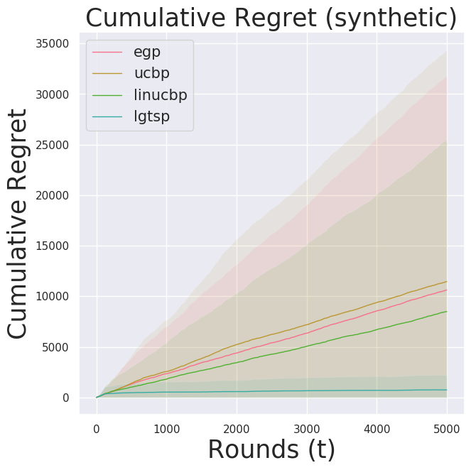
Synthetic (fully observable reward, item context)

We consider a simple hypothetical contextual bandit problem. The true distribution that samples rewards is Gaussian with some predefined variance. Assuming no interactions between actions, we keep the model as an isotropic multivariate Gaussian. As the true model is Gaussian, we expect the thompson sampling poilcy (lgtsp) to perform well.

1
2
3
4
5
6
7
8
9
10
11
12
13
14
15
16
17
18
19
20
21
22
23
24
25
26
27
28
29
30
31
32
33
34

def sample_synthetic(n_samples, n_actions, context_dim, sigma):
    """
    W ~ samples hidden random Matrix of n_actions x context_dim
    x_t ~ samples contexts uniformly from {-5, -4, ..., 4, 5}
    r_t ~ samples rewards from an isotropic multivariate normal
          r_t ~ N(W x_t, \sigma^2 I)

    returns:
        (n_samples)-length stream of data
    """

    np.random.seed(0)
    W = np.random.rand(n_actions, context_dim)
    cov = sigma**2 * np.eye(n_actions)

    x_t_list = []
    r_acts_list = []
    opt_act_list_hidden = []
    mean_list_hidden = []

    for t in range(n_samples):
        x_t = np.random.randint(low=-5, high=5, size=context_dim)
        mean = np.dot(W, x_t)

        r_acts = np.random.multivariate_normal(mean, cov=cov, size=1)
        r_acts = r_acts.squeeze()
        opt_act = np.argmax(mean)

        x_t_list.append(x_t)
        r_acts_list.append(r_acts)
        opt_act_list_hidden.append(opt_act)
        mean_list_hidden.append(mean)

    return x_t_list, r_acts_list, opt_act_list_hidden, mean_list_hidden

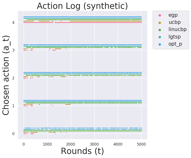
As expected, lgtsp outperformed baselines.

Other baselines especially linucbp did not perform so well because they locked on to one action that it thinks the best and does not get out of it. You can observe that in the action distribution plot below.

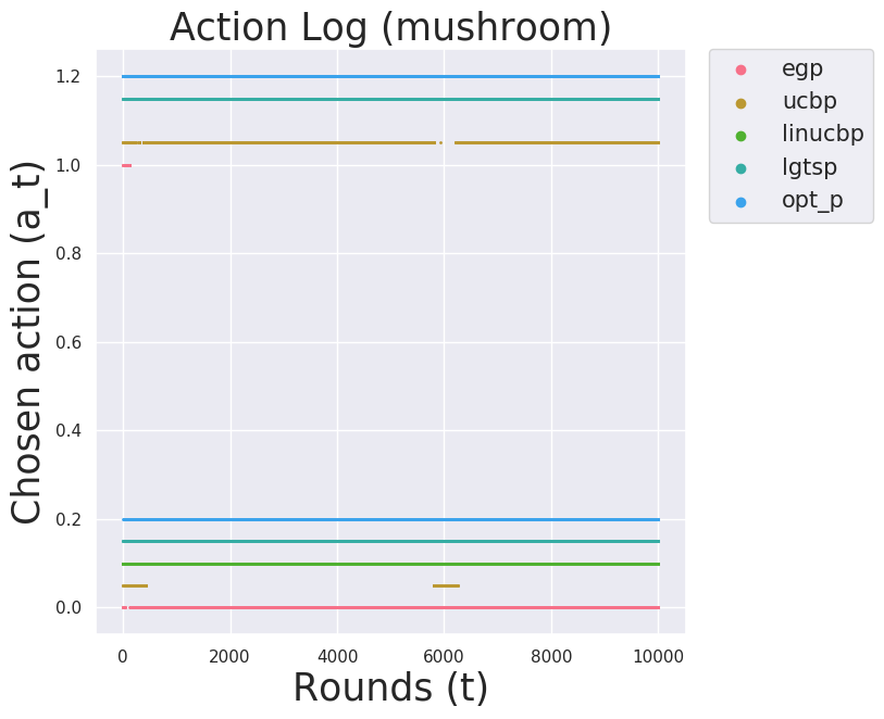
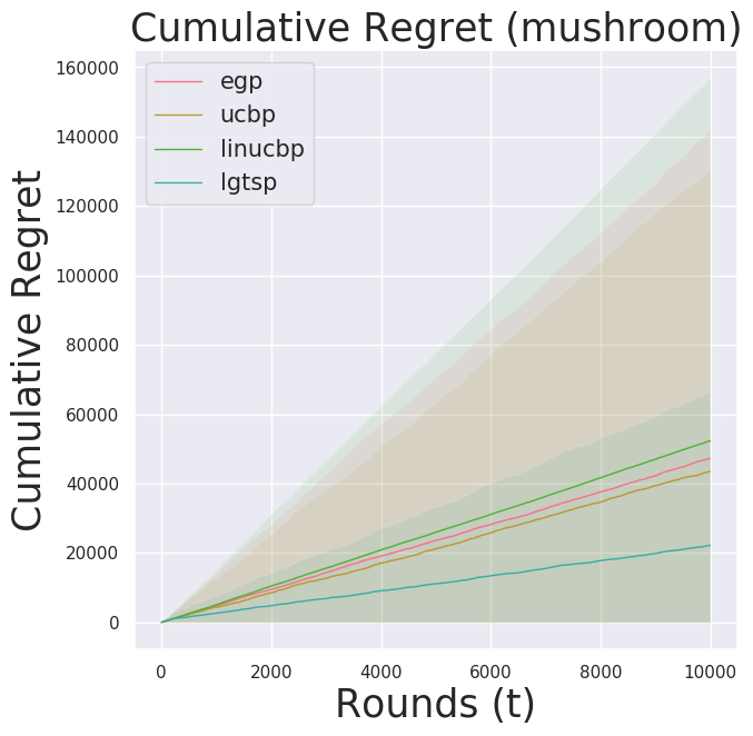
Mushroom (fully observable rewards, item context)

Mushroom consists of 8,124 hypothetical mushroom datapoints that show features (item context) and whether each is poisonous/edible. I modeled the reward distribution similar to the paper where +10.0 for eating a good mushroom, -35.0 for eating a bad mushroom with a 30% chance, still +10.0 with 70% (bad mushroom but lucky), and 0.0 for not eating. The optimal policy would eat only good mushrooms and not take the risk with bad mushrooms. Good and bad mushrooms are in an almost equal proportion. Of course, whether a mushroom is good or bad is hidden (except for opt_p).

1
2
3
4
5
6
7
8
9
10
11
12
13
14
15
16
17
18
19
20
21
22
23
24
25
26
27
28
29
30
31
32
33
34
35
36
37
38
39
40
41
42
43
44
45

def sample_mushroom(X, y,
                    n_mushrooms,
                    r_eat_good,
                    r_eat_bad_lucky,
                    r_eat_bad_unlucky,
                    r_eat_bad_lucky_prob,
                    r_no_eat
                    ):
    """
    ask for n mushrooms
    """
    n, d = X.shape
    indices = np.random.choice(np.arange(n), size=n_mushrooms)

    contexts = X[indices, :]

    # hidden info for the oracle (described below)
    is_poisonous_hidden = y[indices]
    is_edible_hidden = (~y[indices].astype(bool)).astype(int)

    r_no_eats = r_no_eat * np.ones(n_mushrooms)
    r_eats = np.zeros(n_mushrooms)
    # y_i == 1 => bad
    r_eats += r_eat_good * is_edible_hidden
    # y_i == 0 ==> good
    r_eat_bad = np.random.choice([r_eat_bad_lucky, r_eat_bad_unlucky],
                                 p=[r_eat_bad_lucky_prob, 1-r_eat_bad_lucky_prob],
                                 size=n_mushrooms)
    r_eats += r_eat_bad * is_poisonous_hidden

    E_r_no_eat = r_no_eat
    E_r_eat_bad = r_eat_bad_lucky * r_eat_bad_lucky_prob +\
                  r_eat_bad_unlucky * (1 - r_eat_bad_lucky_prob)

    if E_r_no_eat > E_r_eat_bad:
        # eat good and not eat bad
        opt_acts_hidden = is_edible_hidden
    else:
        # take risks: always eat
        opt_acts_hidden = np.ones(n_mushrooms, dtype=int)

    # hidden info, not to be given to an agent
    r_acts = np.hstack((r_no_eats[:, None], r_eats[:, None]))

    return contexts, r_acts, opt_acts_hidden, is_poisonous_hidden

We observe again lgtsp outperfoming baselines. It is quite surprising linucbp performed so poorly. Perhaps there is a bug in the code (recall, this is an intermediate report).

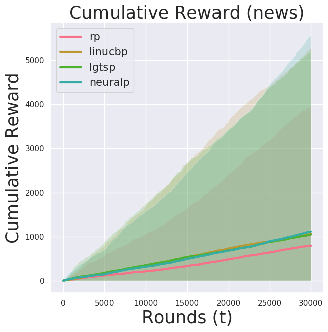
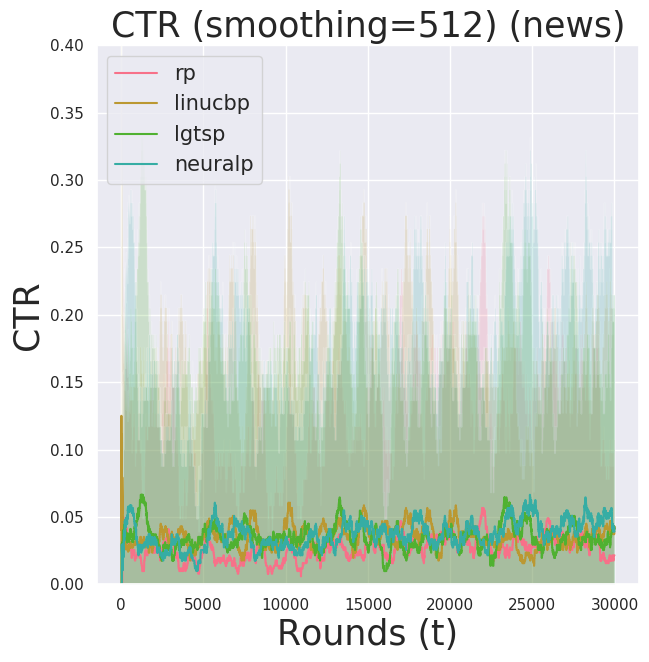
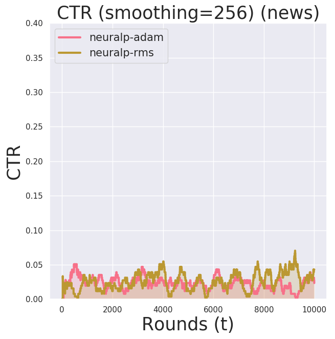
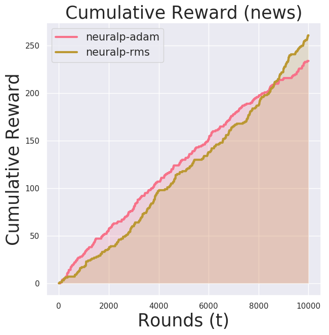
Yahoo Click Log Data (partially observable reward, user+item context)

Yahoo! Front Page Today Module User Click Log Dataset that features a log data for ~45 Million user visit events. For each user visit event, we have features available for the article shortlist (the candidate article pool) and user features. Crucially, the shortlist elements change over time so the algorithm must learn to adapt to a new action set. This is a partially observable reward problem because we do not have the data for the counterfactuals and instead know what article in the shortlist was displayed to the user and whether the user clicked it or not. If we use an on-policy algorithm, the data points we can use is only when our policy’s recommendation matches the chosen article in the data.

Since the behavior policy was a uniform random policy for roughly 20 actions at each time step, the effective sample rate (the rate at which samples could be used for training) was roughly at 5%. This means, in order to compute training over n=10000, we have to evaluate approximately 200,000 points and reject the rest.

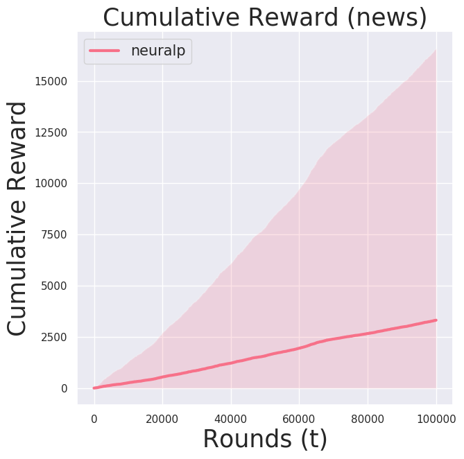
Notice now the y-axis is cumulative reward. Since this is a partially observable reward problem we cannot compute the regret.

Due to computational costs (both theoretically and practically—I run my experiments on EC2 Spot Instances), I ran neuralp for $n=100000$ for now. I observed a high variance in the performance of neuralp (the shaded region). It seemed there is a bad local optimum it tends to get stuck at.

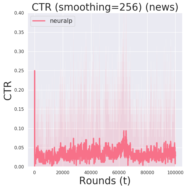
There wasn’t a significant difference in the learning performance between Adam and RMSProp.

Source Code

Check out the source code for more details.